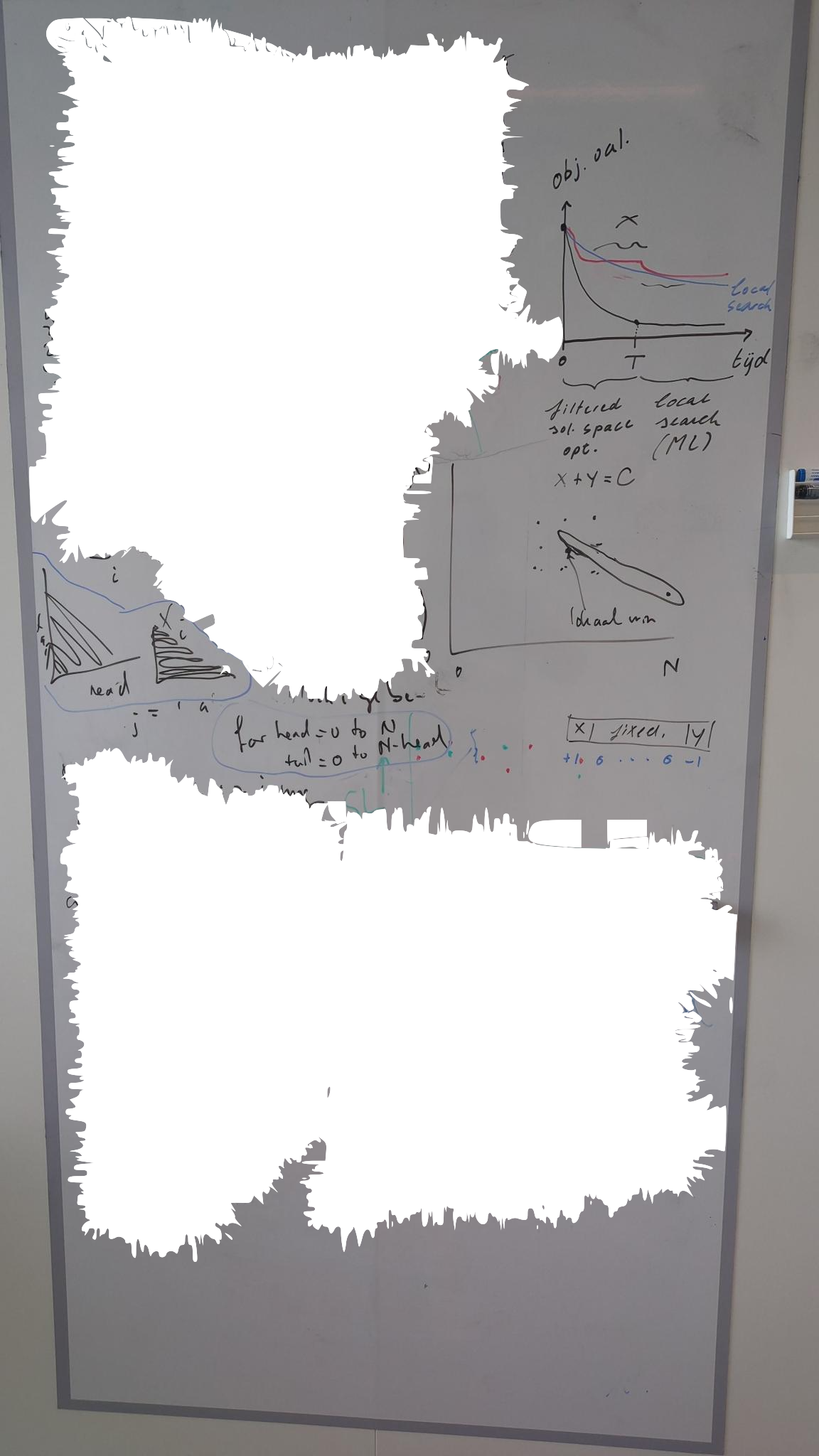
Compare speed local search strategies (with stopping time 1 minute):
Strategy 1: Filtered solution space, starting at S = T = 0 (or lowest possible values) and iteratively adding 1 to each side. Then standard local search.
Code
total =0stop =3while total <= stop:for s inrange(total +1): t = total - sprint(f"Start = {s}, Tail = {t}") total +=1
Strategy 2: Standard local search, with same starting point as in strategy 1.
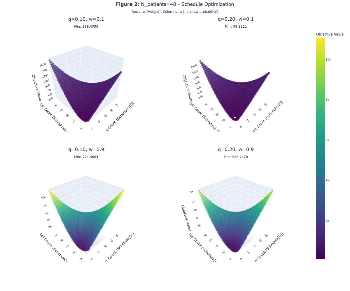
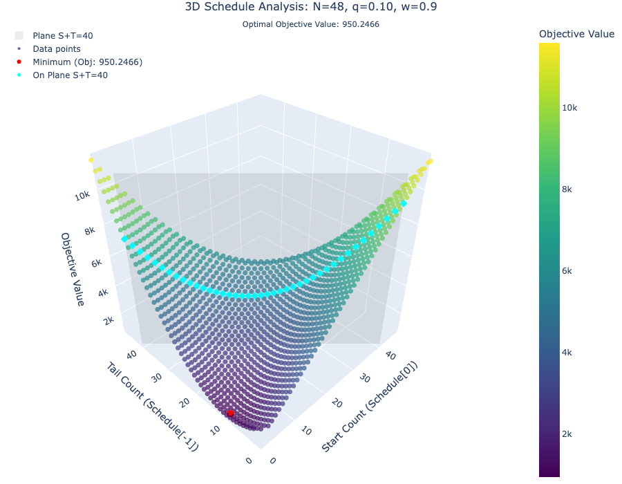
Q: When we limit \(S + T = C\) to what extend does the multimodularity feature hold?
Suggested Plan of Approach (based on Joost’s input)
To address the question of whether the multimodularity (or convexity) feature holds when \(S+T=C\):
Experimental Investigation of Convexity:
Action: Conduct a series of experiments to empirically test for convexity.
Parameters: Vary the value of C and other instance parameters.
Objective: Observe if the convex relationship (like the light blue line in the current visualizations) persists across different settings.
Consistent observation of convexity across varied parameters strengthens the hypothesis.
Finding even a single counterexample would disprove general convexity under these conditions.
Note: Remember that for a given C, you are effectively dealing with a single variable problem (e.g., varying S determines T). This simplifies the experimental setup and analysis.
Formal Proof Attempts (if experimental evidence is supportive):
If experiments suggest convexity holds, attempt a formal proof. Two potential avenues:
Avenue 1 (Direct Proof): Attempt to prove convexity directly from its mathematical definition, following the approach sketched by Ger.
Avenue 2 (Adapt Existing Proofs): Investigate whether the proof arguments from Ger’s existing article can be adapted or still apply within this specific “filtered solution space” context (where \(S+T=C\)).
Key Insight: The reduction to a single variable for a fixed C should simplify the proof structure.
Explore Generalization: Consider a more generalized model by introducing a “curve between the extremes” for patient distribution, rather than just a linear division.
New Parameter: The degree or nature of this curve could become a third parameter, refining the S and T parameters. This is for inspiration and potential future enhancements, not an immediate priority.