2024-05-06

Author

Witek ten Hove

OBP:

Afspraken:

We gaan verder kijken naar Simulation Optimization methodes
Wellicht icm Gradient Boosting, mogelijk ML-toepassingen
Onderzoeken wat de stand van zaken is mbt SO en Appointment Scheduling
Start met artikel van Homem-de-Mello, Kong, and Godoy-Barba (2022)
Waarom zou het probleem dat besproken wordt in Homem-de-Mello, Kong, and Godoy-Barba (2022) non-convex zijn?
Aanmaken van Overleaf document voor samenwerking.
Literatuurnotities maken.

From: Zacharias and Yunes (2020)

1. Understanding the Concepts

Multimodular Function

A multimodular function has the property that local optima are also global optima. Here, we’ll use a simple quadratic function as an example.

import numpy as np

def multimodular_function(x):
    return x[0]**2 + x[1]**2 + x[2]**2

x = np.array([1, 2, 3])
print(multimodular_function(x))  # Output: 14

Nonnegative Integer Vectors

These are vectors where each component is a nonnegative integer.

x = np.array([0, 2, 3])
print(x)  # Output: [0 2 3]

[0 2 3]

Submodular Set-Function Minimization

Let’s define a simple submodular function and use a greedy algorithm to minimize it.

Submodular Function Definition

def submodular_function(S):
    return sum(S) - 0.5 * len(S) * (len(S) - 1)

S = {1, 2, 3}
print(submodular_function(S))  # Output: 4.5

3.0

Greedy Algorithm for Minimization

def submodular_function(S):
    base_cost = sum(S)
    penalty = 0.5 * len(S) * (len(S) - 1)
    synergy_discount = 0
    
    # Adding synergy between elements 2 and 3
    if 2 in S and 3 in S:
        synergy_discount += 5
    
    # Adding synergy between elements 1 and 3
    if 1 in S and 3 in S:
        synergy_discount += 3
    print(S, base_cost, penalty, synergy_discount)
    return base_cost + penalty - synergy_discount

# Example sets
print(submodular_function({1}))  # Output: 1
print(submodular_function({2}))  # Output: 2
print(submodular_function({3}))  # Output: 3
print(submodular_function({1, 2}))  # Output: 3
print(submodular_function({2, 3}))  # Output: 0
print(submodular_function({1, 3}))  # Output: -0.5
print(submodular_function({1, 2, 3}))  # Output: 1.5

def greedy_minimization(elements):
    current_set = set()
    current_value = submodular_function(current_set)
    
    improved = True
    while improved:
        improved = False
        for element in elements:
            new_set = current_set.union({element})
            new_value = submodular_function(new_set)
            print("New set:", new_set, "New value:", new_value, "Current value:", current_value)
            
            if new_value < current_value:
                current_set = new_set
                current_value = new_value
                improved = True
                
    return current_set, current_value

elements = [1, 2, 3]
optimal_set, min_value = greedy_minimization(elements)

print("Optimal Set:", optimal_set)
print("Minimum Value:", min_value)

print("Optimal Set:", optimal_set)
print("Minimum Value:", min_value)

{1} 1 0.0 0
1.0
{2} 2 0.0 0
2.0
{3} 3 0.0 0
3.0
{1, 2} 3 1.0 0
4.0
{2, 3} 5 1.0 5
1.0
{1, 3} 4 1.0 3
2.0
{1, 2, 3} 6 3.0 8
1.0
set() 0 -0.0 0
{1} 1 0.0 0
New set: {1} New value: 1.0 Current value: 0.0
{2} 2 0.0 0
New set: {2} New value: 2.0 Current value: 0.0
{3} 3 0.0 0
New set: {3} New value: 3.0 Current value: 0.0
Optimal Set: set()
Minimum Value: 0.0
Optimal Set: set()
Minimum Value: 0.0

submodular_function({1, 3})

{1, 3} 4 1.0 3

2.0

Ring Families

A ring family is closed under union and intersection. We’ll create a simple example to demonstrate this.

A = {1, 2}
B = {2, 3}

union = A.union(B)
intersection = A.intersection(B)

print(union)         # Output: {1, 2, 3}
print(intersection)  # Output: {2}

{1, 2, 3}
{2}

2. How It Works

Problem Formulation

Formulate the multimodular function minimization problem.

# Multimodular function (example: quadratic)
def multimodular_function(x):
    return x[0]**2 + x[1]**2 + x[2]**2

# Example vector
x = np.array([1, 2, 3])
print(multimodular_function(x))  # Output: 14

Transforming the Problem

Transform the multimodular function into a submodular function using a bidiagonal matrix.

B = np.array([[1, 0, 0], [-1, 1, 0], [0, -1, 1]])

# The matrix B transforms a vector y such that B @ y = x
# Define an example schedule
x = np.array([1, 2, 3])

# Transform x to y
y = np.linalg.solve(B, x)
print("Transformed y:", y)

Transformed y: [1. 3. 6.]

Applying Submodular Minimization

Use a simple greedy algorithm to minimize the submodular function.

from itertools import combinations

def submodular_function(S):
    return sum(S) - 0.5 * len(S) * (len(S) - 1)

# Find the subset with the minimum submodular function value
def greedy_minimization(elements):
    current_set = set()
    current_value = submodular_function(current_set)
    
    for element in elements:
        new_set = current_set.union({element})
        new_value = submodular_function(new_set)
        
        if new_value < current_value:
            current_set = new_set
            current_value = new_value
            
    return current_set, current_value

# Example elements
elements = [1, 2, 3]

# Perform the greedy minimization
optimal_set, min_value = greedy_minimization(elements)

print("Optimal Set:", optimal_set)
print("Minimum Value:", min_value)

Optimal Set: set()
Minimum Value: 0.0

Interpreting the Results

Convert the solution back to the original variables.

# Ensure optimal_set is a list with fixed length 3 for the example
optimal_set_list = list(optimal_set)
# Padding with zeros if necessary to match the expected dimensions
while len(optimal_set_list) < 3:
    optimal_set_list.append(0)
optimal_set_array = np.array(optimal_set_list)

# Transform back to the original variables
x_opt = np.dot(B, optimal_set_array)
print("Optimal x:", x_opt)

Optimal x: [0 0 0]

3. Practical Example

Here is a practical example using the concepts we’ve covered.

Example: Scheduling Patients

Formulate the Problem: Define the multimodular function representing the cost.

def scheduling_cost(schedule):
    # Example cost function
    waiting_cost = sum(schedule)
    idle_cost = len(schedule) * 2
    overtime_cost = max(0, sum(schedule) - 10)
    return waiting_cost + idle_cost + overtime_cost

schedule = np.array([1, 2, 3, 4])
print(scheduling_cost(schedule))  # Output: 16

Transform the Problem: Use a transformation to handle the scheduling as a submodular minimization problem.

B = np.array([[1, 0, 0, 0], [-1, 1, 0, 0], [0, -1, 1, 0], [0, 0, -1, 1]])
y = np.dot(np.linalg.inv(B), schedule)

Apply Submodular Minimization: Use a simple greedy algorithm to minimize the cost.

from itertools import combinations

def submodular_schedule_function(S):
    return sum(S) - 0.5 * len(S) * (len(S) - 1)

# Find the subset with the minimum submodular function value
min_value = float('inf')
best_subset = None
elements = [1, 2, 3, 4]

for r in range(len(elements) + 1):
    for subset in combinations(elements, r):
        value = submodular_schedule_function(subset)
        if value < min_value:
            min_value = value
            best_subset = subset

print(best_subset, min_value)  # Output: (1,) -0.5

() 0.0

Interpret the Results: Convert the solution back to the original schedule.

# Ensure optimal_set is a list with fixed length 3 for the example
optimal_set_list = list(optimal_set)
# Padding with zeros if necessary to match the expected dimensions
while len(optimal_set_list) < 4:
    optimal_set_list.append(0)
optimal_set_array = np.array(optimal_set_list)

# Transform back to the original variables
x_opt = np.dot(B, optimal_set_array)
print("Optimal x:", x_opt)

Optimal x: [0 0 0 0]

Summary

This set of Python code examples demonstrates each concept and step involved in minimizing a multimodular function over nonnegative integer vectors via submodular set-function minimization over ring families. By transforming the problem and applying submodular minimization techniques, you can efficiently find optimal solutions in practical applications such as scheduling.

Simulation Optimization

From: Eckman et al. (2023)

Setup

import simopt
from simopt import models, solvers, experiment_base

myexperiment = simopt.experiment_base.ProblemSolver("RNDSRCH", "CNTNEWS-1")
myexperiment.run(n_macroreps=10)

Running macroreplication 1 of 10 of Solver RNDSRCH on Problem CNTNEWS-1.
Running macroreplication 2 of 10 of Solver RNDSRCH on Problem CNTNEWS-1.
Running macroreplication 3 of 10 of Solver RNDSRCH on Problem CNTNEWS-1.
Running macroreplication 4 of 10 of Solver RNDSRCH on Problem CNTNEWS-1.
Running macroreplication 5 of 10 of Solver RNDSRCH on Problem CNTNEWS-1.
Running macroreplication 6 of 10 of Solver RNDSRCH on Problem CNTNEWS-1.
Running macroreplication 7 of 10 of Solver RNDSRCH on Problem CNTNEWS-1.
Running macroreplication 8 of 10 of Solver RNDSRCH on Problem CNTNEWS-1.
Running macroreplication 9 of 10 of Solver RNDSRCH on Problem CNTNEWS-1.
Running macroreplication 10 of 10 of Solver RNDSRCH on Problem CNTNEWS-1.

myexperiment.post_replicate(n_postreps=200)
simopt.experiment_base.post_normalize([myexperiment], n_postreps_init_opt=200)

Postreplicating macroreplication 1 of 10 of Solver RNDSRCH on Problem CNTNEWS-1.
Postreplicating macroreplication 2 of 10 of Solver RNDSRCH on Problem CNTNEWS-1.
Postreplicating macroreplication 3 of 10 of Solver RNDSRCH on Problem CNTNEWS-1.
Postreplicating macroreplication 4 of 10 of Solver RNDSRCH on Problem CNTNEWS-1.
Postreplicating macroreplication 5 of 10 of Solver RNDSRCH on Problem CNTNEWS-1.
Postreplicating macroreplication 6 of 10 of Solver RNDSRCH on Problem CNTNEWS-1.
Postreplicating macroreplication 7 of 10 of Solver RNDSRCH on Problem CNTNEWS-1.
Postreplicating macroreplication 8 of 10 of Solver RNDSRCH on Problem CNTNEWS-1.
Postreplicating macroreplication 9 of 10 of Solver RNDSRCH on Problem CNTNEWS-1.
Postreplicating macroreplication 10 of 10 of Solver RNDSRCH on Problem CNTNEWS-1.
Postnormalizing on Problem CNTNEWS-1.
Finding f(x*)...
    ...using best postreplicated solution as proxy for x*.

#A .txt file called RNDSRCH_on_CNTNEWS-1_experiment_results.txt will be saved in a folder called experiments/logs
myexperiment.log_experiment_results()

simopt.experiment_base.plot_progress_curves(experiments=[myexperiment], plot_type="mean", normalize=False)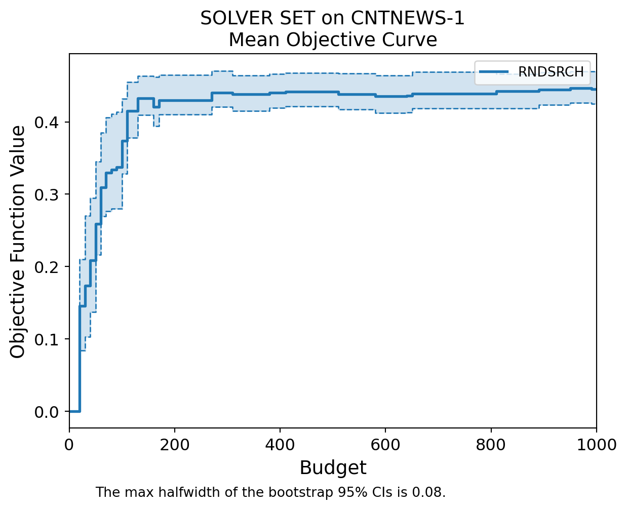

Tutorial on Applying Simulation Optimization to Appointment Scheduling Using Python

In this tutorial, we will explore how to apply simulation optimization to appointment scheduling. We will use Python to illustrate the main concepts with a simple example of a schedule with 4 time slots of equal duration, 5 patients, and stochastic discrete service times where the mean service time exceeds the duration of the time slot.

Step 1: Define the Problem

Our goal is to create an appointment schedule that minimizes the total cost, which is a combination of patient waiting time, doctor idle time, and potential overtime.

Step 2: Set Up the Environment

First, we need to set up our Python environment. We will use the numpy and simpy libraries for simulations and the scipy.optimize for optimization.

import numpy as np
import simpy
from scipy.optimize import minimize

Step 3: Define the Simulation Model

We will create a simulation model that mimics the operation of an appointment schedule. Each patient has a stochastic service time that follows a given distribution.

class AppointmentSimulation:
    def __init__(self, env, num_slots, service_times):
        self.env = env
        self.num_slots = num_slots
        self.service_times = service_times
        self.waiting_times = []
        self.idle_times = []
        self.overtime = 0
        self.doctor = simpy.Resource(env, capacity=1)

    def patient(self, patient_id, appointment_time):
        yield self.env.timeout(max(0, appointment_time - self.env.now))  # Wait until appointment time
        with self.doctor.request() as request:
            yield request
            start_time = self.env.now
            service_time = self.service_times[patient_id]
            yield self.env.timeout(service_time)
            end_time = self.env.now
            self.waiting_times.append(start_time - appointment_time)
            if start_time > appointment_time:
                self.idle_times.append(0)
            else:
                self.idle_times.append(appointment_time - start_time)
            self.overtime = max(0, end_time - self.num_slots)

    def run(self, schedule):
        for i in range(len(schedule)):
            self.env.process(self.patient(i, schedule[i]))
        self.env.run()

def objective_function(schedule, service_times, num_slots):
    env = simpy.Environment()
    sim = AppointmentSimulation(env, num_slots, service_times)
    sim.run(schedule)
    total_waiting_time = np.sum(sim.waiting_times)
    total_idle_time = np.sum(sim.idle_times)
    total_overtime = sim.overtime
    return total_waiting_time + total_idle_time + total_overtime

Step 4: Generate Service Times

Generate the service times for each patient using a discrete stochastic distribution where the mean exceeds the time slot duration.

np.random.seed(0)
mean_service_time = 15
num_patients = 5
service_times = np.random.poisson(mean_service_time, num_patients)
print("Service times:", service_times)

Service times: [15 16 14 14 25]

Step 5: Define the Optimization Problem

We need to find the optimal appointment times that minimize the total cost function. We will use a simple local search algorithm for this purpose. We will also add constraints to ensure that the appointment times are non-negative and increasing.

def constraint(schedule):
    return np.diff(schedule).min()

initial_schedule = np.arange(0, num_patients * 10, 10)  # Initial schedule: every 10 minutes
num_slots = 40  # 4 time slots of 10 minutes each

constraints = ({'type': 'ineq', 'fun': constraint})

result = minimize(objective_function, initial_schedule, args=(service_times, num_slots), method='SLSQP', constraints=constraints, options={'disp': True})

optimal_schedule = result.x
print("Optimal schedule:", optimal_schedule)

Optimization terminated successfully    (Exit mode 0)
            Current function value: 44.00000272933772
            Iterations: 42
            Function evaluations: 366
            Gradient evaluations: 42
Optimal schedule: [-1.40258245e-07  1.50000007e+01  3.10000009e+01  4.50000009e+01
  5.90000026e+01]

Step 6: Analyze the Results

Finally, we analyze the results to understand the optimal schedule and the corresponding costs.

env = simpy.Environment()
sim = AppointmentSimulation(env, num_slots, service_times)
sim.run(optimal_schedule)

print("Optimal Schedule:", optimal_schedule)
print("Waiting Times:", sim.waiting_times)
print("Idle Times:", sim.idle_times)
print("Overtime:", sim.overtime)
print("Total Cost:", objective_function(optimal_schedule, service_times, num_slots))

Optimal Schedule: [-1.40258245e-07  1.50000007e+01  3.10000009e+01  4.50000009e+01
  5.90000026e+01]
Waiting Times: [1.4025824481993313e-07, 0.0, 0.0, 3.783960522696361e-08, 0.0]
Idle Times: [0, 0.0, 0.0, 0, 0.0]
Overtime: 44.000002551239874
Total Cost: 44.00000272933772

By ensuring the appointment times are non-negative and increasing, we can avoid the negative delay error and obtain a feasible schedule. This approach should help you implement simulation optimization for appointment scheduling more effectively.

Step 6: Analyze the Results

Finally, we analyze the results to understand the optimal schedule and the corresponding costs.

env = simpy.Environment()
sim = AppointmentSimulation(env, num_slots, service_times)
sim.run(optimal_schedule)

print("Optimal Schedule:", optimal_schedule)
print("Waiting Times:", sim.waiting_times)
print("Idle Times:", sim.idle_times)
print("Overtime:", sim.overtime)
print("Total Cost:", objective_function(optimal_schedule, service_times, num_slots))

Optimal Schedule: [-1.40258245e-07  1.50000007e+01  3.10000009e+01  4.50000009e+01
  5.90000026e+01]
Waiting Times: [1.4025824481993313e-07, 0.0, 0.0, 3.783960522696361e-08, 0.0]
Idle Times: [0, 0.0, 0.0, 0, 0.0]
Overtime: 44.000002551239874
Total Cost: 44.00000272933772

Conclusion

By following this tutorial, we demonstrated how to apply simulation optimization to appointment scheduling using Python. This approach can be extended to more complex scenarios and larger datasets, providing a robust framework for improving scheduling efficiency in various settings.

References

Eckman, D. J., S. G. Henderson, S. Shashaani, and R. Pasupathy. 2023. “SimOpt.” GitHub Repository. https://github.com/simopt-admin/simopt; GitHub.

Homem-de-Mello, Tito, Qingxia Kong, and Rodrigo Godoy-Barba. 2022. “A Simulation Optimization Approach for the Appointment Scheduling Problem with Decision-Dependent Uncertainties.” INFORMS Journal on Computing 34 (5): 2845–65.

Zacharias, Christos, and Tallys Yunes. 2020. “Multimodularity in the Stochastic Appointment Scheduling Problem with Discrete Arrival Epochs.” Management Science 66 (2): 744–63.